Pulse duration calibration¶

A device that drives a fractional iSWAP, $\mathrm{iSWAP}^{k}$, can calibrate any duration $k$ of a full iSWAP, but each calibration costs effort. Synthesis costs answer which durations to calibrate for the circuits the device runs. The workload here is a six-qubit quantum Fourier transform (QFT), including its final bit-reversal SWAPs, and the score of a set of durations is the summed synthesis cost of the QFT’s two-qubit blocks.

import numpy as np
from qiskit import QuantumCircuit
from qiskit.circuit.library import QFTGate, iSwapGate
from gulps.analysis.coverage import two_qubit_blocks

workload = QuantumCircuit(6)
workload.append(QFTGate(6), range(6))
blocks = two_qubit_blocks(workload)
base = iSwapGate()
print(f"Two-qubit blocks: {len(blocks)}")

Two-qubit blocks: 18

Fifteen blocks are controlled-phase gates and three are SWAPs. The controlled-phase angles $\pi/2,\pi/4,\pi/8,\pi/16,\pi/32$ occur five, four, three, two, and one times.

Costs are durations in units of a full iSWAP, so $\mathrm{iSWAP}^{k}$ costs $k$. Under the cost model, each layer of single-qubit gates around the pulses also costs $\ell$, the local_layer_cost of the device. Here $\ell=0.1$.

One duration for the workload¶

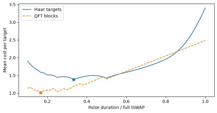
With one calibrated duration, the QFT costs least at $\mathrm{iSWAP}^{1/6}$.

from gulps.analysis.calibration import strength_sweep

local_layer_cost = 0.1
qft_sweep = strength_sweep(
    base, local_layer_cost=local_layer_cost, workload=workload
)
print(f"Duration fraction: {qft_sweep.best[0]:.4f}")
print(f"Total QFT block cost: {qft_sweep.best[1]:.4f}")

Duration fraction: 0.1667
Total QFT block cost: 18.3333

The sweep tests the fractions in gulps.analysis.calibration.GRID. Pass strengths= to test the durations your device can calibrate.

Workload against Haar-random targets¶

Typical quantum algorithms do not use a uniform distribution of two-qubit gates. The QFT, for example, uses controlled-phase gates $\mathrm{CP}(\theta)$ at a few small angles, plus SWAPs. Without a workload, strength_sweep calibrates for Haar-random targets, which are uniform over all two-qubit gates, and selects $\sqrt[3]{\mathrm{iSWAP}}$ instead of the $\mathrm{iSWAP}^{1/6}$ it selects when calibrated for the QFT.

from gulps.analysis.coverage import empirical_cost
from gulps.decomposition import GulpsDecomposer

def instruction_set(strengths):
    return GulpsDecomposer(
        [base.power(k) for k in strengths],
        costs=list(strengths),
        local_layer_cost=local_layer_cost,
    )

haar_sweep = strength_sweep(base, local_layer_cost=local_layer_cost)
print(f"Haar-selected duration: {haar_sweep.best[0]:.4f}")
for name, sweep in (("Haar choice", haar_sweep), ("QFT choice", qft_sweep)):
    device = instruction_set([sweep.best[0]])
    print(f"{name}: QFT cost {empirical_cost(device, blocks).total_cost:.4f}")

Haar-selected duration: 0.3333
Haar choice: QFT cost 21.3000
QFT choice: QFT cost 18.3333

On the QFT, the Haar choice costs 21.30 against 18.33, 16% more. The plot shows both sweeps as mean cost per target. Each curve averages over its own targets, so compare durations along one curve.

Plotting code

import matplotlib.pyplot as plt

colors = {"Haar targets": "C0", "QFT blocks": "C1"}
fig, ax = plt.subplots(figsize=(7, 3.6), layout="constrained")
for name, sweep, count, style, marker in (
    ("Haar targets", haar_sweep, 1, "-", "o"),
    ("QFT blocks", qft_sweep, len(blocks), "--", "s"),
):
    values = np.asarray(sweep.costs) / count
    ax.plot(sweep.strengths, values, linestyle=style, color=colors[name], label=name)
    k, cost = sweep.best
    ax.scatter(k, cost / count, marker=marker, color=colors[name], zorder=3)
ax.set(xlabel="Pulse duration / full iSWAP", ylabel="Mean cost per target")
ax.legend()
plt.close(fig)

$Cost of fractional iSWAP instruction sets. The solid Haar curve has its minimum at one-third duration; the dashed QFT curve has its minimum at one-sixth.$

Sensitivity to the local-layer cost¶

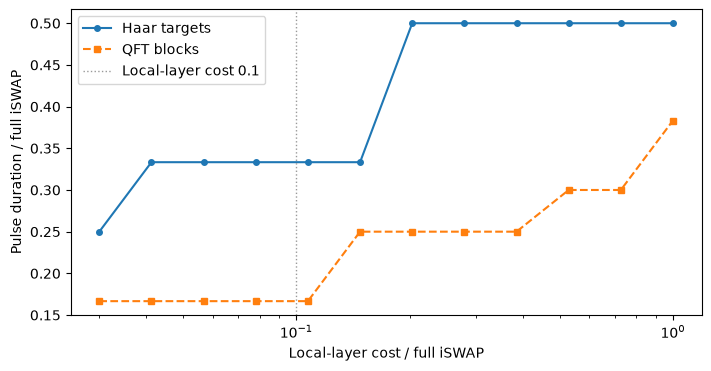
The local-layer cost is a property of the hardware, and the duration to calibrate depends on it. As $\ell$ grows, fewer and longer pulses win, because each pulse adds a local layer. At every $\ell$, the QFT selects a shorter pulse than Haar-random targets, because its small rotations need little interaction time.

layer_costs = np.geomspace(0.03, 1.0, 12)
selected = {
    name: [
        strength_sweep(base, local_layer_cost=ell, workload=sample).best[0]
        for ell in layer_costs
    ]
    for name, sample in (("Haar targets", None), ("QFT blocks", workload))
}

Plotting code

fig, ax = plt.subplots(figsize=(7, 3.6), layout="constrained")
for (name, strengths), style in zip(selected.items(), ("o-", "s--")):
    ax.plot(layer_costs, strengths, style, color=colors[name], markersize=4, label=name)
ax.axvline(local_layer_cost, color="0.6", linestyle=":", linewidth=1,
           label=f"Local-layer cost {local_layer_cost}")
ax.set(
    xscale="log",
    xlabel="Local-layer cost / full iSWAP",
    ylabel="Pulse duration / full iSWAP",
)
ax.legend()
plt.close(fig)

Selected iSWAP duration against local-layer cost on a log axis. Circles with a solid line show Haar targets; squares with a dashed line show QFT blocks. Both select longer pulses at higher local-layer costs, and the QFT curve lies below the Haar curve at every local-layer cost.

Calibrate more durations¶

Each extra calibrated duration lowers the QFT cost, by less each time. calibrate adds the duration that lowers the cost most, then re-chooses each earlier one.

from gulps.analysis.calibration import calibrate

pair = calibrate(
    base, budget=2, local_layer_cost=local_layer_cost, workload=workload
)
print("Duration fractions:", [round(k, 4) for k in pair.strengths])
print(f"Total QFT block cost: {pair.cost:.4f}")

Duration fractions: [0.1667, 0.5]
Total QFT block cost: 16.5333

A second duration, $\sqrt{\mathrm{iSWAP}}$, lowers the cost from 18.3333 to 16.5333 without saving any interaction time. It saves pulses, and with them local layers:

print(f"{'Calibration':13} {'Pulses':>6} {'Interaction':>13} {'Local layers':>15} {'Total':>7}")
choices = {"One duration": [qft_sweep.best[0]], "Two durations": pair.strengths}
table = {}
for name, strengths in choices.items():
    sequences = instruction_set(strengths).select(blocks)
    pulses = sum(len(gates) for _, gates in sequences)
    total = sum(cost for cost, _ in sequences)
    local = (pulses + len(blocks)) * local_layer_cost
    table[name] = (pulses, total - local)
    print(f"{name:13} {pulses:6} {total - local:13.4f} {local:15.4f} {total:7.4f}")

Calibration   Pulses   Interaction    Local layers   Total
One duration      62       10.3333          8.0000 18.3333
Two durations     44       10.3333          6.2000 16.5333

Each SWAP used nine $\mathrm{iSWAP}^{1/6}$ pulses and now uses three $\sqrt{\mathrm{iSWAP}}$ pulses. The controlled-phase blocks keep the short pulses.

A further duration can serve blocks that no chosen duration handles cheaply. GRID lacks the short durations that the smallest QFT rotations need, so the code also calibrates from an expanded grid, GRID plus $1/64, 1/32, 1/16, 1/8$. With six durations from it, the QFT reaches the cost of the best continuous-duration construction.

from gulps.analysis.calibration import GRID

budgets = calibrate(
    base, budget=6, local_layer_cost=local_layer_cost, workload=workload
)
tailored = (1 / 64, 1 / 32, 1 / 16, 1 / 8, 1 / 4, 1 / 2)
expanded = calibrate(
    base, budget=6, strengths=sorted(set(GRID) | set(tailored)),
    local_layer_cost=local_layer_cost, workload=workload,
)
reference = empirical_cost(instruction_set(tailored), blocks).total_cost
print("Durations    Default grid    Expanded grid")
for count, original, extended in zip(range(1, 7), budgets.budget_costs, expanded.budget_costs):
    print(f"{count:9} {original:15.4f} {extended:16.4f}")
print(f"Continuous-duration optimum: {reference:.5f}")

Durations    Default grid    Expanded grid
        1         18.3333          18.3333
        2         16.5333          16.1000
        3         15.3667          15.2000
        4         14.9667          14.4500
        5         14.9667          14.2625
        6         14.9667          14.2312
Continuous-duration optimum: 14.23125

Plotting code

fig, ax = plt.subplots(figsize=(7, 4), layout="constrained")
counts = np.arange(1, 7)
ax.plot(counts, budgets.budget_costs, "s--", color=colors["QFT blocks"],
        label="Default duration grid")
ax.plot(counts, expanded.budget_costs, "o-", color=colors["QFT blocks"],
        label="Grid + QFT-tailored durations")
ax.axhline(reference, color="0.3", linestyle=":", label="Continuous-duration optimum")
ax.set(xlabel="Number of calibrated durations", ylabel="Total QFT block cost",
       xticks=counts, ylim=(13.9, 18.7))
ax.legend(loc="upper right", fontsize=9)
plt.close(fig)

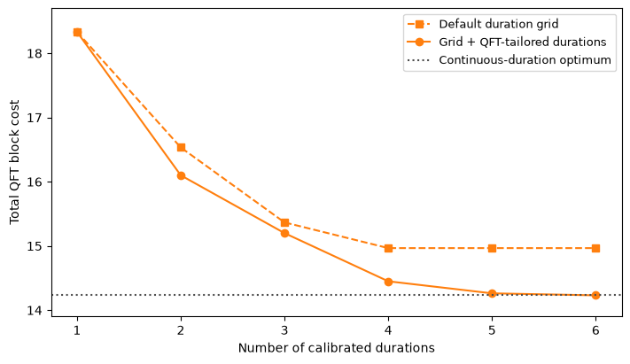
Total QFT cost falls as the number of calibrated durations grows from one to six. The default grid levels off near 14.97 at four durations. Including shorter QFT-tailored durations reaches 14.45 at four and the reference cost 14.23125 at six.

On the expanded grid, four durations come within 1.5% of the optimum.

Continuous-duration optimum

A controlled-phase block of angle $\theta$ uses two $\mathrm{iSWAP}^{a}$ pulses with $a=\theta/(2\pi)$. A local echo between them cancels one interaction axis and adds the other. Each SWAP uses three $\sqrt{\mathrm{iSWAP}}$ pulses along the three pairs of axes. The QFT then takes 39 pulses and 57 local layers, at total cost 14.23125.

No set of durations does better. The interaction time of a controlled-phase block is at least $2a$, and that of SWAP at least $3/2$ (Theorem 1 and Eq. 16 of Vidal, Hammerer, and Cirac). A controlled-phase block needs at least two fractional-iSWAP pulses, and SWAP at least three. The construction meets both the interaction-time and the pulse-count bounds, so it also has the fewest local layers.

SWAP exchanges the two single-qubit factors of any local gate. A two-pulse implementation would therefore require one pulse to be locally equivalent to SWAP times the inverse of the other. For a pulse fraction $k\in[0,1]$, that product has Weyl coordinates $(1/2,(1-k)/2,(1-k)/2)$. No fractional iSWAP, whose coordinates are $(r/2,r/2,0)$, has this class. By the same comparison, one fractional iSWAP cannot implement a nonzero controlled-phase class $(a,0,0)$.

Greedy against exhaustive search¶

For two durations, the greedy pair is within 1.6% of the best grid pair for the QFT and is the best grid pair for Haar-random targets. Scoring every pair of GRID fractions takes 1,540 instruction sets per objective and several minutes. docs/_scripts/calibration_grid.py saves the result:

def pair_landscapes() -> tuple[np.ndarray, dict[str, np.ndarray]]:
    """Mean cost of every GRID pair, on Haar targets and on the QFT blocks."""
    grid = np.asarray(GRID)
    landscapes = {}
    for name in ("Haar targets", "QFT blocks"):
        costs = np.full((len(grid), len(grid)), np.nan)
        for i, first in enumerate(grid):
            for j in range(i, len(grid)):
                device = instruction_set(sorted({float(first), float(grid[j])}))
                costs[j, i] = (
                    coverage_report(device).expected_cost
                    if name == "Haar targets"
                    else empirical_cost(device, blocks).expected_cost
                )
        landscapes[name] = costs
    return grid, landscapes

import json

with open("docs/_scripts/calibration_grid.json") as file:
    data = json.load(file)
grid = np.asarray(data["grid"])
landscapes = {name: np.array(costs, dtype=float) for name, costs in data["costs"].items()}

qft_costs = landscapes["QFT blocks"]
j, i = np.unravel_index(np.nanargmin(qft_costs), qft_costs.shape)
exact_cost = qft_costs[j, i] * len(blocks)
print("Best QFT pair:", [round(float(k), 4) for k in (grid[i], grid[j])])
print(f"Total QFT block cost: {exact_cost:.4f}")
print(f"Greedy cost above optimum: {100 * (pair.cost / exact_cost - 1):.2f}%")

haar_pair = calibrate(base, budget=2, local_layer_cost=local_layer_cost)
print("Greedy Haar pair:", [round(k, 4) for k in haar_pair.strengths])

Best QFT pair: [0.1333, 0.25]
Total QFT block cost: 16.2667
Greedy cost above optimum: 1.64%

Greedy Haar pair: [0.3333, 0.4833]

Plotting code

greedy_pairs = {"Haar targets": haar_pair, "QFT blocks": pair}
fig, axes = plt.subplots(
    1, 2, figsize=(7.5, 3.6), layout="constrained", sharex=True, sharey=True
)
extent = (grid[0] - 1 / 120, grid[-1] + 1 / 120) * 2
for ax, (name, costs) in zip(axes, landscapes.items()):
    j, i = np.unravel_index(np.nanargmin(costs), costs.shape)
    im = ax.imshow(
        costs / np.nanmin(costs), origin="lower", extent=extent,
        cmap="viridis_r", vmin=1, vmax=1.3,
    )
    ax.plot(grid[i], grid[j], "*", color="white", markeredgecolor="black",
            markersize=13, label="Grid minimum")
    ax.plot(*greedy_pairs[name].strengths, "o", markerfacecolor="none",
            markeredgecolor="red", markersize=12, label="calibrate")
    ax.set(title=name, xlabel="First pulse duration / full iSWAP")
    ax.legend(fontsize=9, loc="lower right")
axes[0].set_ylabel("Second pulse duration / full iSWAP")
fig.colorbar(im, ax=axes, label="Mean cost / grid minimum", shrink=0.8, extend="max")
plt.close(fig)

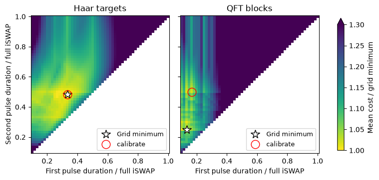
$Two triangular cost maps for pairs of fractional iSWAP durations, with stars marking grid minima and rings marking the pairs calibrate chose. The markers coincide for Haar targets but differ for QFT blocks. Each panel normalizes costs to its own minimum.$

The best QFT pair drops $\sqrt{\mathrm{iSWAP}}$. Its SWAPs take six $\mathrm{iSWAP}^{1/4}$ pulses instead of three, but each $\mathrm{CP}(\pi/2)$ takes two pulses instead of three, and the other controlled-phase blocks use the shorter $\mathrm{iSWAP}^{2/15}$.

Compile with the calibrated durations¶

The compiled QFT uses all six durations, 39 pulses, as many as the continuous-duration optimum. A pulse $\mathrm{iSWAP}^{k}$ appears as an xx_plus_yy gate with first parameter $-\pi k$.

from collections import Counter
from qiskit.transpiler import PassManager
from qiskit.transpiler.passes import (
    HighLevelSynthesis, Unroll3qOrMore, Optimize1qGatesDecomposition,
)
from gulps.transpiler import GulpsDecompositionPass

decomposer = instruction_set(expanded.strengths)
pipeline = PassManager([
    HighLevelSynthesis(),
    Unroll3qOrMore(),
    GulpsDecompositionPass(decomposer),
    Optimize1qGatesDecomposition(basis=["u"]),
])
compiled = pipeline.run(workload)
pulses = Counter(
    round(-float(op.operation.params[0]) / np.pi, 6)
    for op in compiled.data if op.operation.name == "xx_plus_yy"
)
for k, count in sorted(pulses.items()):
    print(f"Fraction {k:.6f}: {count} pulses")

Fraction 0.015625: 2 pulses
Fraction 0.031250: 4 pulses
Fraction 0.062500: 6 pulses
Fraction 0.125000: 8 pulses
Fraction 0.250000: 10 pulses
Fraction 0.500000: 9 pulses