How synthesis works

Selection and construction both work with reachable regions.

Sentence selection

The running example uses two native instructions, \(A=\sqrt{\mathrm{CX}}\) and \(B=\sqrt[3]{\mathrm{iSWAP}}\), with costs 90 and 120, and a target with Weyl coordinates \((3/8,5/16,1/8)\).

from qiskit.circuit.library import CSXGate, iSwapGate
from gulps.analysis.region import ReachableRegion
from gulps.decomposition import GulpsDecomposer
from gulps.invariants import LocalEquivalenceClass

native_gates = [CSXGate(label="A"), iSwapGate().power(1 / 3)]
native_gates[1].label = "B"
classes = dict(zip("AB", LocalEquivalenceClass.from_unitaries(native_gates)))
costs = {"A": 90, "B": 120}
target = LocalEquivalenceClass((3 / 8, 5 / 16, 1 / 8))

print(f"{'Sentence':10} {'Cost':>4}  Reaches target")
for sentence in ("", "A", "B", "AA", "AB", "BB", "AAA", "AAB"):
    region = ReachableRegion.of(classes[name] for name in sentence)
    cost = sum(costs[name] for name in sentence)
    print(f"{sentence or 'Local only':10} {cost:4}  {region.reaches(target)}")

Sentence   Cost  Reaches target
Local only    0  False
A            90  False
B           120  False
AA          180  False
AB          210  False
BB          240  False
AAA         270  False
AAB         300  True

No sentence cheaper than AAB reaches the target. From AA, appending A misses it and appending B reaches it. Local gates cost nothing in this example, and any four native gates cost at least 360, so no longer sentence can improve on AAB at 300.

The table lists one ordering of each combination of gates. Because the local gates between instructions are arbitrary, AAB, ABA, and BAA have the same reachable region, although their bare matrix products can differ.

The decomposer selects the same sentence:

decomposer = GulpsDecomposer(native_gates, costs=[90, 120])
cost, selected = decomposer.select(target)
print(cost, [gate.name for gate in selected])

300.0 ['csx', 'csx', 'xx_plus_yy']

The cost-ordered search tree

Each sentence extends its prefix by one native gate, so AA is the prefix of AAB. Candidates wait in a queue ordered by cost, and the first one whose region contains the target is the cheapest. To generate each combination once, a sentence only appends instructions at or after its last one in cost order: A grows into AA or AB, and B only into BB.

A candidate is pruned, with all its extensions, when one cheaper sentence contains its region and permits the same extensions, because its last instruction comes no later in cost order.

With B at cost 120, BB costs 240 and leaves the queue before AAA at 270, so AAA cannot prune it. Raising B to 150 makes BB cost 300. AAA contains the region of BB and ends in A, the first instruction in the order, so the search prunes BB. The same rule prunes ABB by AAAA and AABB by AAAAA.

from IPython.display import display
from gulps.analysis.coverage import coverage_report

for b_cost in (120, 150):
    tree_report = coverage_report(GulpsDecomposer(native_gates, costs=[90, b_cost]))
    display(tree_report.plot_tree(["A", "B"]))

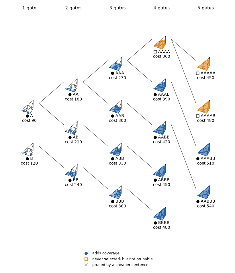
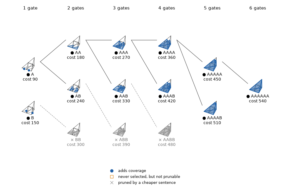
Each node draws a sentence’s reachable region, and an edge joins it to its prefix. A child region need not contain its parent’s region, because the child must use the added instruction.

Orange sentences, such as AAAA in the first tree, are never selected: the union of cheaper regions already contains their region. No single cheaper sentence contains it, though, and testing containment in a union is expensive, so the search keeps them and extends them.

Coverage across targets

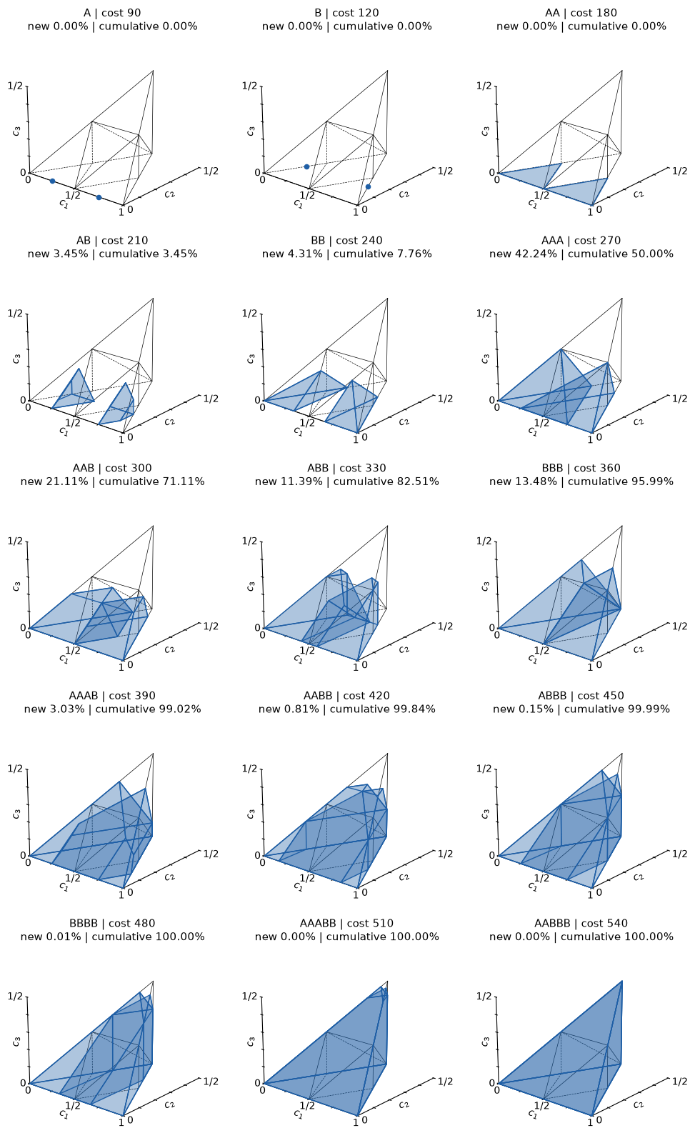
The regions fill the Weyl chamber as cost grows. In each panel, new is the Haar mass that no cheaper sentence reaches and cumulative is the mass of all regions so far.

report = coverage_report(decomposer)
report.plot()

Reachable-region composition

Every region, for any sentence length, is cut out by fourteen lower bounds on sums of four ordered phases \(x\ge y\ge z\ge w\), which are linear in the Weyl coordinates. Appending an instruction updates the bounds by one max-plus step. The reachability calculation derives both.

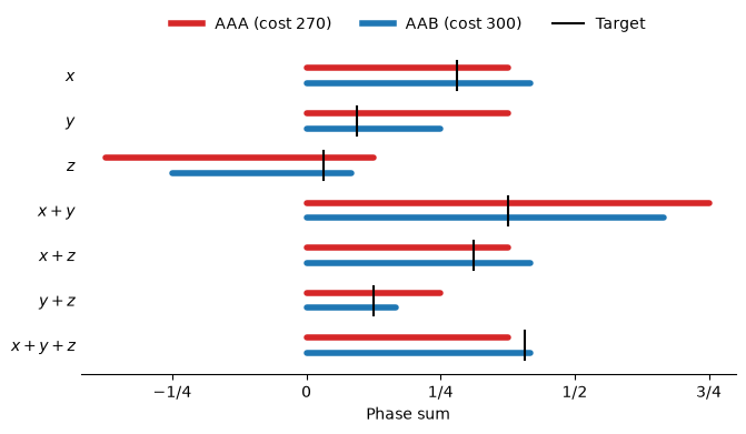
Complementary sums pair into seven intervals, which the figure draws for AAA and AAB. The example target has phases \((x,y,z,w)=(9/32,3/32,1/32,-13/32)\), so \(x+y+z=13/32\). The AAA region requires \(x+y+z\le3/8\), so AAA misses the target. AAB admits this value and passes the other six intervals.

Each class has two global-phase representatives, and the target must pass all seven intervals for one of them. The figure uses the direct representative. reaches() also tests the reflected one, which AAA misses as well.

import numpy as np

def phase_sums(weyl):
    c1, c2, c3 = np.asarray(weyl).T
    x = (c1 + c2 - c3) / 2
    y = (c1 - c2 + c3) / 2
    z = (-c1 + c2 + c3) / 2
    return np.array([x, y, z, x + y, x + z, y + z, x + y + z])

values = phase_sums(target.weyl)
intervals = {}
for sentence in ("AAA", "AAB"):
    region = ReachableRegion.of(classes[name] for name in sentence)
    sums = phase_sums(region.vertices)  # linear, so extremes are at vertices
    intervals[sentence] = (sums.min(axis=1), sums.max(axis=1))
    print(f"{sentence}: x+y+z in [{sums[-1].min():.4f}, {sums[-1].max():.4f}], "
          f"target {values[-1]:.4f}")

AAA: x+y+z in [0.0000, 0.3750], target 0.4062
AAB: x+y+z in [0.0000, 0.4167], target 0.4062

Plotting code

import matplotlib.pyplot as plt

from matplotlib.lines import Line2D

labels = ["$x$", "$y$", "$z$", "$x+y$", "$x+z$", "$y+z$", "$x+y+z$"]
rows = np.arange(len(labels))
interval_figure, ax = plt.subplots(figsize=(6.6, 3.8), layout="constrained")
handles = []
for sentence, shift, color in (("AAA", -0.17, "tab:red"), ("AAB", 0.17, "tab:blue")):
    lower, upper = intervals[sentence]
    ax.hlines(rows + shift, lower, upper, color=color, linewidth=4, capstyle="round")
    cost = sum(costs[name] for name in sentence)
    handles.append(Line2D([], [], color=color, linewidth=4, label=f"{sentence} (cost {cost})"))
for row, value in zip(rows, values):
    ax.plot([value, value], [row - 0.32, row + 0.32], color="black", linewidth=1.5, zorder=3)
handles.append(Line2D([], [], color="black", linewidth=1.5, label="Target"))
ax.set_yticks(rows, labels)
ax.invert_yaxis()
ax.set_xticks([-1 / 4, 0, 1 / 4, 1 / 2, 3 / 4], ["−1/4", "0", "1/4", "1/2", "3/4"])
ax.set_xlim(-0.42, 0.8)
for side in ("top", "right", "left"):
    ax.spines[side].set_visible(False)
ax.tick_params(axis="y", length=0)
ax.set_xlabel("Phase sum")
ax.legend(handles=handles, loc="lower center", bbox_to_anchor=(0.5, 1.0),
          ncol=3, frameon=False)
plt.close(interval_figure)

Local-gate construction

A region that contains the target shows that the sentence reaches the target’s local-equivalence class. To implement the target matrix, GULPS also needs the single-qubit gates and the global phase. It first chooses the class reached after each prefix, then solves for the local gates between consecutive classes.

Let \(G_i\) be the class of the \(i\)-th native instruction, \(\mathcal R_i\) the region of the first \(i\), and \(C_i\) the class they reach, in Weyl coordinates. The target fixes the final class \(C_n\). Working backward, each preceding class must lie in the prefix region and in the region reached from \(C_i\) by the inverse of the last instruction:

\[C_{i-1}\in\mathcal R_{i-1}\cap\operatorname{Reach}(C_i,G_i^{-1}).\]

If \(G_i\) has ordered eigenphases \((x,y,z,w)\), its inverse has \((-w,-z,-y,-x)\).

Both regions bound the same fourteen sums, so their intersection keeps the larger lower bound of each. Any point in the intersection works: being in the backward region connects it to \(C_i\), and being in the prefix region means the earlier gates can reach it, so no look-ahead is needed. GULPS takes the point with the smallest \(x\), then the largest \(y\), then the smallest \(z\), and repeats the step back to the first gate.

The next figure shows the repeated intersections for the sentence BBBB. Read the panels backward from the target: each chosen class becomes the target of the next, shorter prefix.

from gulps.analysis.viz.polytope_viz import plot_waypoints

backward_decomposer = GulpsDecomposer([native_gates[1]], costs=[120])
backward_target = LocalEquivalenceClass((0.42, 0.35, 0.28))
plot_waypoints(backward_decomposer, backward_target.matrix)

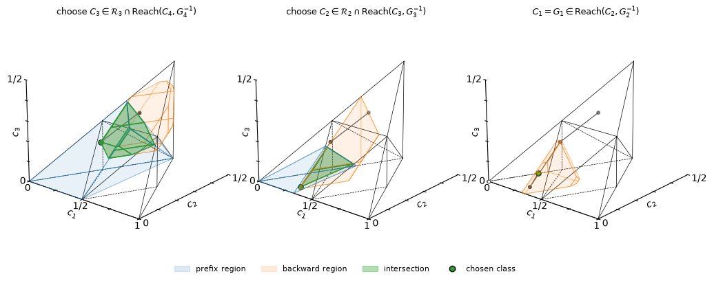
In each panel, the filled intersection holds the allowed predecessors, the outlined point is the chosen class, and the gray path joins the classes already fixed. In the last panel the prefix region is the single point \(C_1=G_1\), so no choice remains.

For AAB, only the class after AA is free, and its intersection has a closed form. The AA prefix has phases \((s,t,-t,-s)\). Intersecting its bounds with the backward region gives the trapezoid

\[\frac{23}{96}\le s\le\frac14, \qquad \frac1{32}\le t\le s-\frac7{48}.\]

The upper bound on \(s\) comes from AA, and the backward region gives the lower bounds on \(s\), \(t\), and \(s-t\). The selection rule takes the smallest \(s=23/96\), then the largest \(t=3/32\), which gives Weyl coordinates \(C_2=(s+t,s-t,0)=(1/3,7/48,0)\). This is a chosen class, not an extra native instruction. It splits the construction into two steps:

\[\begin{split}(A,A)&\longrightarrow C_2,\\ (C_2,B)&\longrightarrow (3/8,5/16,1/8).\end{split}\]

Recovering the middle local gate

Each step has a middle local gate that takes \(C_{i-1}\) and \(G_i\) to \(C_i\), because \(C_i\) lies in the region of that pair. The can_sandwich solver finds this gate by solving the inverse spectral problem below. The unknowns are the two single-qubit gates \(u_i\) and \(v_i\) between the prefix and the next native instruction.

Plotting code

from qiskit import QuantumCircuit
from qiskit.circuit import Gate

segment = QuantumCircuit(2)
segment.append(Gate(r"$\mathrm{CAN}(C_{i-1})$", 2, []), [0, 1])
segment.append(Gate("$u_i$", 1, []), [0])
segment.append(Gate("$v_i$", 1, []), [1])
segment.append(Gate(r"$\mathrm{CAN}(G_i)$", 2, []), [0, 1])
segment_figure = segment.draw("mpl")
plt.close(segment_figure)

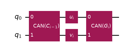
One input stands for the whole accumulated prefix, so a sentence of \(n\) native gates needs \(n-1\) two-gate solves. For monodromy coordinates \(m=(x,y,z)\), with \(w=-x-y-z\), the canonical gate in the magic basis is

\[D(m)=\operatorname{diag} (e^{i\pi y},e^{i\pi x},e^{i\pi w},e^{i\pi z}).\]

For a class \(C\), \(D(C)\) means \(D\) at the monodromy coordinates of \(C\). The solver finds \(O\in SO(4)\) such that

\[\operatorname{spec}\!\left(D(G_i)^2 O D(C_{i-1})^2 O^T\right) =\operatorname{spec}\!\left(sD(C_i)^2\right),\qquad s\in\{-1,1\}.\]

The sign \(s\) covers the two global-phase representatives. In the computational basis, \(O\) is the middle local gate \(V_i=u_i\otimes v_i\). To recover the full target matrix, solve_with_factors takes \((G_i,C_{i-1},C_i)\) and also returns endpoint factors and a phase:

\[D(G_i)O D(C_{i-1})=e^{i\eta_i}L_i D(C_i)R_i,\qquad L_i,R_i\in SO(4).\]

Assembly of the local factors

In the computational basis, the factorization for each step is

\[\operatorname{CAN}(G_i)V_i\operatorname{CAN}(C_{i-1}) =L_i\operatorname{CAN}(C_i)R_i e^{i\eta_i}.\]

GULPS assembles the canonical sentence first and substitutes the native instructions afterward, which keeps the class-dependent solve separate from the local factors of each native instruction. Write the accumulated canonical prefix as \(P_{i-1}=E_{i-1}\operatorname{CAN}(C_{i-1})F_{i-1}e^{i\phi_{i-1}}\). For the first gate, \(C_1=G_1\), \(E_1=F_1=I\), and \(\phi_1=0\). For each later gate, GULPS inserts the layer \(W_i=V_iE_{i-1}^{-1}\), which cancels the previous left factor:

\[\operatorname{CAN}(G_i)W_iP_{i-1} =L_i\operatorname{CAN}(C_i)R_iF_{i-1} e^{i(\eta_i+\phi_{i-1})}.\]

The endpoint factors and phase update as

\[E_i=L_i,\qquad F_i=R_iF_{i-1},\qquad \phi_i=\phi_{i-1}+\eta_i.\]

Next, write each native instruction as \(\widetilde G_i=\ell_i\operatorname{CAN}(G_i)r_i e^{i\gamma_i}\). Replacing each canonical gate by \(\widetilde G_i\) changes the layer between \(\widetilde G_{i-1}\) and \(\widetilde G_i\) to

\[M_i=r_i^{-1}W_i\ell_{i-1}^{-1}.\]

The physical sentence then has endpoint factors \(\widetilde E_n=\ell_nE_n\) and \(\widetilde F_n=F_nr_1\), and phase \(\widetilde\phi_n=\phi_n+\sum_i\gamma_i\). For a target \(U=T_L\operatorname{CAN}(C_n)T_R e^{i\theta}\), GULPS attaches the final local layers

\[K_{\mathrm{after}}=T_L\widetilde E_n^{-1},\qquad K_{\mathrm{before}}=\widetilde F_n^{-1}T_R,\]

and corrects the global phase by \(\theta-\widetilde\phi_n\). The circuit then equals the target matrix.