The reachability calculation

GULPS describes the reachable region of a sentence by fourteen lower bounds. Each bound applies to the sum of one nonempty proper subset of the four eigenphases of the Cartan double, defined in the next section. Appending a native gate to the sentence updates the fourteen bounds with a fixed table of 72 quantum Littlewood–Richardson rules.

The calculation extends a two-gate result of Peterson, Crooks, and Smith, Two-Qubit Circuit Depth and the Monodromy Polytope, to sentences of any length.

Shared mathematical setup

from fractions import Fraction

import matplotlib.pyplot as plt
import numpy as np
from qiskit.circuit.library import CSXGate, CXGate, iSwapGate
from gulps.analysis.region import ReachableRegion
from gulps.invariants import LocalEquivalenceClass

cx = LocalEquivalenceClass.from_unitary(CXGate())
sqrt_iswap = LocalEquivalenceClass.from_unitary(iSwapGate().power(1 / 2))
native_a = LocalEquivalenceClass.from_unitary(CSXGate())
native_b = LocalEquivalenceClass.from_unitary(iSwapGate().power(1 / 3))

Coordinates in which products are tractable

Weyl coordinates describe a single gate, but they are not convenient for computing the class of a product of two gates. Eigenvalues are better suited to products, through the multiplicative version of Horn’s problem, which the two-gate section states. The eigenvalues of a two-qubit gate, however, are not invariants of its class. Local gates \(L\) and \(R\) around \(U\) change its eigenvalues in general, because \(R\) need not equal \(L^{-1}\).

For a real matrix \(X\), orthogonal factors in \(O_LXO_R\) likewise change the eigenvalues of \(X\), but not those of \(XX^T\), which are the squared singular values of \(X\). The Cartan double is the two-qubit analog of \(XX^T\).

In the magic basis, a phased Bell basis, local special unitaries become real orthogonal matrices. Fix \(\det U=1\) (Two global-phase representatives treats the choices) and write \(U_B\) for \(U\) in this basis. Its KAK decomposition is \(U_B=O_L D O_R\), with \(D\) diagonal and \(O_L,O_R\in SO(4)\), and the Cartan double is

\[M(U)=U_B U_B^T =O_L D O_R O_R^T D O_L^T =O_L D^2 O_L^T.\]

The superscript \(T\) is a plain transpose, not a conjugate transpose, so \(O_R O_R^T=I\) removes the right local factor. The left factor only conjugates \(D^2\) and leaves its eigenvalues unchanged. The spectrum of \(M(U)\) therefore depends only on the class of the representative.

Write the eigenvalues as \(e^{2\pi i x},e^{2\pi i y},e^{2\pi i z},e^{2\pi i w}\). The phases are measured in turns, so adding an integer to one of them does not change its eigenvalue. The fundamental alcove picks one representative for each spectrum:

\[x\ge y\ge z\ge w,\qquad x+y+z+w=0,\qquad x-w\le1.\]

The first three phases \((x,y,z)\) are the monodromy coordinates of the representative. The fourth phase, \(w=-x-y-z\), stays in the notation because the inequalities treat all four phases alike.

The phases are linear in the Weyl coordinates \(c=(c_1,c_2,c_3)\). When they satisfy the alcove conditions, each Weyl coordinate is the sum of two phases, so a bound on a pair sum of phases reads directly as a bound on a Weyl coordinate:

\[c_1=x+y,\qquad c_2=x+z,\qquad c_3=y+z,\]

\[(x,y,z,w)=\frac12( c_1+c_2-c_3,\ c_1-c_2+c_3,\ -c_1+c_2+c_3,\ -c_1-c_2-c_3).\]

def phases(weyl):
    c1, c2, c3 = weyl
    return np.array([
        c1 + c2 - c3, c1 - c2 + c3,
        -c1 + c2 + c3, -c1 - c2 - c3,
    ]) / 2

print("√iSWAP phases:", phases(sqrt_iswap.weyl).round(3))

√iSWAP phases: [ 0.25  0.    0.   -0.25]

Two global-phase representatives

A gate has four global-phase representatives, the determinant-one matrices \(U\) divided by each fourth root of \(\det U\). They differ by the factors \(1,i,-1,-i\). The transpose does not conjugate a scalar, so \(M(sU)=s^2M(U)\). Multiplying by \(-1\) leaves the Cartan double unchanged, while multiplying by \(i\) negates it. The four representatives therefore give two spectra, and a reachability test must accept either one.

Negating the double shifts every eigenphase by \(1/2\) modulo integers. Returning the shifted phases to the alcove gives the reflection

\[\rho(x,y,z,w)= (z+1/2,\ w+1/2,\ x-1/2,\ y-1/2).\]

Math detail: the reflected phases lie in the alcove

The reflected phases are ordered because \(x-w\le1\), and their spread \(1+z-y\) is at most one. Applying \(\rho\) twice returns the original spectrum.

In Weyl coordinates the reflection reads

\[\rho(c_1,c_2,c_3)=(1-c_1,c_2,-c_3).\]

def rho(spectrum):
    x, y, z, w = spectrum
    return np.array([z + 0.5, w + 0.5, x - 0.5, y - 0.5])

identity = phases((0, 0, 0))
print("Identity spectra:", identity, rho(identity))

Identity spectra: [0. 0. 0. 0.] [ 0.5  0.5 -0.5 -0.5]

A sentence of \(n\) gates has \(4^n\) choices of global-phase representatives, four per gate. The factors \(1,i,-1,-i\) collect into one power of \(i\) on the product, and only its parity changes the product’s Cartan double. The choices therefore reach two regions, related by \(\rho\). On this page, the direct representative of a sentence takes, for each gate, the representative whose phases the Weyl-coordinate formula above gives, and the reflected representative is its \(\rho\) partner. A target class is reachable, up to global phase, when its spectrum or its \(\rho\) partner lies in the region of the direct representative. reaches() checks the target against both region and region.rho.

Two gates as a multiplicative Horn problem

The Cartan double of a two-gate circuit has the same spectrum as a product of the two gates’ doubles, with one factor rotated by the middle local layer. The reach of a two-gate sentence is therefore a question about the eigenvalues of products.

Absorb the local factors at the ends of each native gate into the adjacent free local layers. In the magic basis, the nonlocal part of the circuit then has the form \(V=D_b O D_a\), where \(D_a,D_b\) are diagonal canonical gates and \(O\in SO(4)\) represents the middle local layer. Its Cartan double is

\[M(V)=D_b O D_a^2 O^T D_b,\]

and conjugating it by \(D_b\) gives

\[D_b M(V)D_b^{-1}=D_b^2 O D_a^2 O^T.\]

Similarity preserves eigenvalues, so \(M(V)\) has the spectrum of \(D_b^2\) times \(O D_a^2 O^T\). Both factors have fixed spectra, and the middle layer \(O\) sets only their relative eigenvectors.

The multiplicative Horn problem asks which spectra a product of two special unitaries can have when the eigenvalues of each factor are fixed and the eigenvectors are free. The original problem of Horn asks the same question for sums of Hermitian matrices. Klyachko and Knutson and Tao proved that its answer is a polytope cut out by linear inequalities. Agnihotri and Woodward and Belkale solved the multiplicative problem. Peterson, Crooks, and Smith call the answer the monodromy polytope. Its points are the triples \((a,b,\delta)\) of alcove points such that some special unitaries with eigenphases \(a\) and \(b\) have a product with eigenphases \(\delta\). Their Theorem 23 lists its faces as linear inequalities, one per entry of a fixed table derived below, and their Corollary 25 proves that a two-gate sentence reaches a target exactly when the target’s spectrum, or its \(\rho\) partner, satisfies them. On the rest of this page, \(\delta\) denotes the spectrum of a product.

A warm-up with 2×2 matrices

For 2-by-2 matrices the eigenvector freedom can be eliminated by hand. The answer already has the shape of the general result, a region bounded by linear inequalities. Here \(U\) and \(V\) are 2×2 special unitaries standing in for Cartan doubles.

Let \(U\) and \(V\) have eigenvalues \(e^{\pm2\pi i a}\) and \(e^{\pm2\pi i b}\), with \(a,b\in[0,1/2]\). In terms of unit vectors \(\mathbf n,\mathbf m\) and the Pauli matrices,

\[\begin{split}U&=\cos(2\pi a)I+i\sin(2\pi a)\,\mathbf n\cdot\boldsymbol\sigma,\\ V&=\cos(2\pi b)I+i\sin(2\pi b)\,\mathbf m\cdot\boldsymbol\sigma.\end{split}\]

\(U\) rotates the Bloch sphere about the axis \(\mathbf n\), and \(V\) rotates it about \(\mathbf m\). The eigenvectors of each matrix are the two states on its axis. The product has eigenvalues \(e^{\pm2\pi i\delta}\), with \(\delta\in[0,1/2]\). Since \((\mathbf n\cdot\boldsymbol\sigma)(\mathbf m\cdot\boldsymbol\sigma) =(\mathbf n\cdot\mathbf m)I+i(\mathbf n\times\mathbf m)\cdot\boldsymbol\sigma\) and the Pauli matrices are traceless, half the trace of the product is

\[\cos(2\pi\delta)=\cos(2\pi a)\cos(2\pi b) -s\sin(2\pi a)\sin(2\pi b), \qquad s=\mathbf n\cdot\mathbf m\in[-1,1].\]

The eigenvectors enter the product spectrum only through \(s\), the cosine of the angle between the two axes, and every \(s\) in \([-1,1]\) occurs. Cosine is monotone on \([0,\pi]\), so the two extreme orientations bound \(\delta\):

\[|a-b|\le\delta\le\min(a+b,\,1-a-b).\]

Written as linear inequalities on the triple \((a,b,\delta)\), these are the inequalities of Peterson, Crooks, and Smith’s Example 24:

\[\delta\ge a-b,\qquad \delta\ge b-a,\qquad \delta\le a+b,\qquad \delta\le1-a-b.\]

The last inequality comes from phases wrapping around the circle. When \(a+b\) exceeds \(1/2\), the eigenvalue pair \(e^{\pm2\pi i(a+b)}\) equals \(e^{\pm2\pi i(1-a-b)}\).

a_demo, b_demo = 1 / 8, 1 / 6
orientations = np.linspace(-1, 1, 501)
cosine = (
    np.cos(2 * np.pi * a_demo) * np.cos(2 * np.pi * b_demo)
    - orientations * np.sin(2 * np.pi * a_demo) * np.sin(2 * np.pi * b_demo)
)
output_phase = np.arccos(np.clip(cosine, -1, 1)) / (2 * np.pi)
expected_interval = (abs(a_demo - b_demo), min(a_demo + b_demo, 1 - a_demo - b_demo))

Plotting code

lo, hi = expected_interval
angle = np.degrees(np.arccos(orientations))
fig, ax = plt.subplots(figsize=(6.4, 3.4), layout="constrained")
ax.plot(angle, output_phase, color="tab:blue", linewidth=2)
ax.axhspan(lo, hi, color="tab:blue", alpha=0.12)
ax.annotate(r"parallel axes: $\delta=a+b$", (0, hi), xytext=(8, 4),
            textcoords="offset points", fontsize=9)
ax.annotate(r"antiparallel axes: $\delta=|a-b|$", (180, lo), xytext=(-8, 6),
            textcoords="offset points", ha="right", fontsize=9)
ax.set_xticks([0, 45, 90, 135, 180], ["0°", "45°", "90°", "135°", "180°"])
ax.set_yticks([0, lo, 1 / 8, 1 / 4, hi], ["0", "1/24", "1/8", "1/4", "7/24"])
ax.set_ylim(0, 0.33)
ax.set(xlabel="Angle between the two rotation axes",
       ylabel=r"Product phase $\delta$")
for side in ("top", "right"):
    ax.spines[side].set_visible(False)
plt.close(fig)

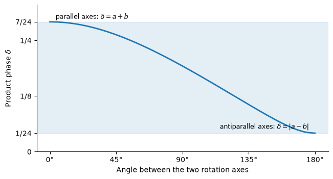
Each factor rotates the Bloch sphere by a fixed amount, and the middle layer only turns one rotation axis relative to the other. The rotations add when the axes are parallel and subtract when they are antiparallel.

With four eigenvalues the relative eigenbasis has too many parameters to eliminate by hand. Theorem 23 of Peterson, Crooks, and Smith does the elimination in general, and its answer is again a list of linear inequalities, now on sums of phases.

From one inequality to fourteen bounds

For a concrete pair, take \(A=\sqrt{\mathrm{CX}}\) followed by \(B=\sqrt[3]{\mathrm{iSWAP}}\). Their Weyl coordinates are \((1/4,0,0)\) and \((1/6,1/6,0)\), so their Cartan-double phases are

\[a=(1/8,1/8,-1/8,-1/8),\qquad b=(1/6,0,0,-1/6).\]

Each inequality of Theorem 23 bounds a sum of output phases from below by a sum of input phases. For a subset \(I\) of the phase positions \(\{x,y,z,w\}\), let \(f_I(a)=\sum_{i\in I}a_i\). For example, \(f_{yw}(a)=a_y+a_w\). Every inequality then has the form

\[f_K(\delta)\ge f_I(a)+f_J(b)-d.\]

The sum of output phases over \(K\) is at least the sum of the first gate’s phases over \(I\) plus the sum of the second gate’s phases over \(J\), less an integer \(d\ge0\). This integer, the quantum degree, accounts for phases wrapping around the circle; the 2×2 bound \(\delta\le1-a-b\) is a rule of degree one. The triples of subsets and their degrees come from a fixed table of 72 rules \((I,J)\to(K,d)\). The table does not depend on the gates, which supply only the phase values.

Take the rule yw + xz -> xy, which has \(d=0\). It gives

\[\delta_x+\delta_y\ge(a_y+a_w)+(b_x+b_z)=0+1/6=1/6.\]

Five other rules also end at \(xy\), each with its own lower bound.

def phase_sum(spectrum, subset):
    return sum(spectrum["xyzw".index(p)] for p in subset)

a_phases = (Fraction(1, 8), Fraction(1, 8), -Fraction(1, 8), -Fraction(1, 8))
b_phases = (Fraction(1, 6), 0, 0, -Fraction(1, 6))

def candidates(rows):
    return {(i, j, d): phase_sum(a_phases, i) + phase_sum(b_phases, j) - d
            for i, j, d in rows}

xy_rows = [("xy", "zw", 0), ("zw", "xy", 0), ("yw", "xz", 0),
           ("xz", "yw", 0), ("yz", "yz", 0), ("xw", "xw", 0)]
xy_candidates = candidates(xy_rows)
beta_xy = max(xy_candidates.values())
for (i, j, d), value in xy_candidates.items():
    print(f"f_{i}(a) + f_{j}(b) = {value}")
print("Strongest:", beta_xy)

f_xy(a) + f_zw(b) = 1/12
f_zw(a) + f_xy(b) = -1/12
f_yw(a) + f_xz(b) = 1/6
f_xz(a) + f_yw(b) = -1/6
f_yz(a) + f_yz(b) = 0
f_xw(a) + f_xw(b) = 0
Strongest: 1/6

All six inequalities hold at once, so their maximum replaces them with one equivalent constraint,

\[x+y\ge\max(1/12,-1/12,1/6,-1/6,0,0)=1/6.\]

Plotting code

def fraction_text(value):
    value = Fraction(value)
    sign = "−" if value < 0 else ""
    if value.denominator == 1:
        return sign + str(abs(value.numerator))
    return f"{sign}{abs(value.numerator)}/{value.denominator}"

ordered = sorted(xy_candidates.items(), key=lambda item: -item[1])
zoom_figure, ax = plt.subplots(figsize=(6.8, 2.9), layout="constrained")
ax.axhline(0, color="0.6", linewidth=0.8, zorder=0)
ax.hlines(0, 1 / 6, 5 / 12, color="tab:blue", linewidth=6, capstyle="round", zorder=1)
ax.text(5 / 12, -0.22, r"$x+y\leq 5/12$", ha="center", va="top",
        fontsize=9, color="tab:blue")
for row, ((i, j, d), value) in enumerate(ordered):
    best = value == beta_xy
    color = "crimson" if best else "0.45"
    height = 0.3 + 0.24 * row
    ax.plot([value, value], [0, height], color=color, linewidth=0.8, linestyle=":")
    ax.plot(value, 0, "o", color=color, markersize=7, zorder=3)
    ax.text(value + 0.006, height,
            rf"$f_{{{i}}}(a)+f_{{{j}}}(b)={fraction_text(value)}$",
            va="center", fontsize=9, color=color)
ax.text(1 / 6, -0.22, r"$x+y\geq 1/6$", ha="center", va="top",
        fontsize=9, color="crimson")
ax.set_ylim(-0.55, 0.3 + 0.24 * len(ordered))
ax.set_yticks([])
ax.set_xticks([-1 / 6, -1 / 12, 0, 1 / 12, 1 / 6, 5 / 12],
              ["−1/6", "−1/12", "0", "1/12", "1/6", "5/12"])
ax.set_xlim(-0.22, 0.5)
for side in ("top", "right", "left"):
    ax.spines[side].set_visible(False)
ax.set_xlabel(r"Output phase sum $x+y$ after AB")
plt.close(zoom_figure)

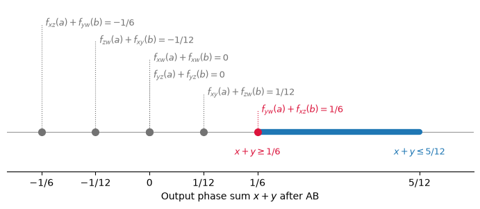
The largest candidate, in red, is the left end of the interval of \(x+y\) values that AB can produce. There are \(\binom41+\binom42+\binom43=4+6+4=14\) nonempty proper subsets of the four phases, and keeping the largest candidate for each gives the fourteen bounds of the theorem:

\[\beta_K=\max_{(I,J)\to(K,d)}\bigl(f_I(a)+f_J(b)-d\bigr).\]

The right end of the blue interval comes from a different output subset. Since \(x+y+z+w=0\), every lower bound on a sum is also an upper bound on the complementary sum. For example,

\[\beta_x\le x\le-\beta_{yzw},\qquad \beta_{xy}\le x+y\le-\beta_{zw}.\]

For AB, six rules end at \(zw\). The rule zw + zw -> zw has degree zero and gives \(f_{zw}(a)+f_{zw}(b)=-1/4-1/6=-5/12\). The other five carry degree one or two and give at most \(-5/6\).

zw_rows = [("zw", "zw", 0), ("yw", "xz", 1), ("xz", "yw", 1),
           ("yz", "xw", 1), ("xw", "yz", 1), ("xy", "xy", 2)]
beta_zw = max(candidates(zw_rows).values())
print(f"{beta_xy} <= c1 <= {-beta_zw}")

1/6 <= c1 <= 5/12

Since \(c_1=x+y\), the direct representative of AB satisfies \(1/6\le c_1\le5/12\). The reflection \(\rho\) sends \(c_1\) to \(1-c_1\), so the reflected representative reaches only \(c_1\ge7/12\). CX has \(c_1=1/2\), between \(5/12\) and \(7/12\), so neither representative reaches it.

mixed = ReachableRegion.of((native_a, native_b))
print("AB reaches B:", mixed.reaches(native_b))
print("AB reaches CX:", mixed.reaches(cx))

AB reaches B: True
AB reaches CX: False

The fourteen lower bounds pair into seven two-sided bounds, on

\[x,\quad y,\quad z,\quad x+y,\quad x+z,\quad y+z,\quad x+y+z.\]

Each two-sided bound confines one phase sum to an interval, and by Theorem 23 a spectrum in the alcove lies in the region of the direct representative exactly when each of its seven phase sums lies in its interval. The figure draws the plane \(c_3=0\), where \(x+y+z=x\), \(z=-y\), and \(y+z=0\), so four intervals remain: those of \(x\), \(y\), \(x+y\), and \(x+z\). Each interval appears as a band between two parallel lines, at the range its phase sum attains on the region.

sum_names = ["x", "y", "z", "w", "x+y", "x+z", "y+z"]

def phase_sums(weyl):
    x, y, z, w = phases(weyl)
    return np.array([x, y, z, w, x + y, x + z, y + z])

at_vertices = np.array([phase_sums(v) for v in mixed.vertices])
lower, upper = at_vertices.min(axis=0), at_vertices.max(axis=0)

c1, c2 = np.meshgrid(np.linspace(0.0005, 0.9995, 500), np.linspace(0.0007, 0.4993, 250))
plane = np.column_stack([c1.ravel(), c2.ravel(), np.zeros(c1.size)])
in_chamber = (c2 <= c1) & (c1 + c2 <= 1)
sums = np.array([phase_sums(p) for p in plane]).reshape(*c1.shape, -1)
in_intervals = np.all((lower <= sums + 1e-12) & (sums <= upper + 1e-12), axis=-1)
inside = mixed.contains(plane).reshape(c1.shape)
disagree = in_chamber & (in_intervals != inside)
print(f"{(in_chamber & inside).sum()} grid points in the region, {disagree.sum()} disagree")

5945 grid points in the region, 0 disagree

Plotting code

from matplotlib.patches import Patch

# Each phase sum as a linear function of (c1, c2) on the plane c3 = 0.
intervals = {"x": (0.5, 0.5), "y": (0.5, -0.5), "x+y": (1, 0), "x+z": (0, 1)}
colors = ["tab:purple", "tab:green", "tab:orange", "tab:brown"]

interval_figure, ax = plt.subplots(figsize=(7, 4.1), layout="constrained")
ax.fill([0, 1, 0.5], [0, 0, 0.5], color="0.95")
ax.plot([0, 1, 0.5, 0], [0, 0, 0.5, 0], color="0.4", linewidth=1)
handles = []
for (name, (n1, n2)), color in zip(intervals.items(), colors):
    k = sum_names.index(name)
    value = np.where(in_chamber, n1 * c1 + n2 * c2, np.nan)
    ax.contourf(c1, c2, (lower[k] <= value) & (value <= upper[k]),
                levels=[0.5, 1.5], colors=[color], alpha=0.13)
    ax.contour(c1, c2, value, levels=[lower[k], upper[k]], colors=[color], linewidths=1.4)
    lo, hi = (fraction_text(Fraction(v).limit_denominator(48)) for v in (lower[k], upper[k]))
    handles.append(Patch(facecolor=color, edgecolor=color, alpha=0.5,
                         label=f"{lo} ≤ ${name}$ ≤ {hi}"))
ax.contourf(c1, c2, in_chamber & inside, levels=[0.5, 1.5], colors=["tab:blue"])
handles.append(Patch(color="tab:blue", label="Region of AB"))
for name, point, offset in (("Identity", (0, 0), (6, 8)),
                            ("B", (1 / 6, 1 / 6), (-14, 6)),
                            ("CX", (1 / 2, 0), (6, 8))):
    ax.scatter(*point, s=40, color="black", zorder=4)
    ax.annotate(name, point, xytext=offset, textcoords="offset points", fontsize=9)
ax.set(xlim=(-0.02, 1.02), ylim=(-0.02, 0.52), xlabel=r"$c_1$", ylabel=r"$c_2$")
ax.set_aspect("equal")
ax.legend(handles=handles, loc="upper right", fontsize=8.5)
plt.close(interval_figure)

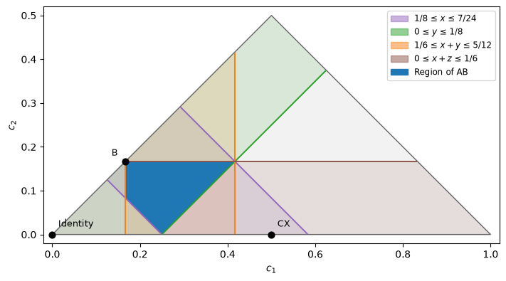
The reflected representative contributes the mirror image of this quadrilateral under \(c_1\mapsto1-c_1\), which also misses CX.

Where the 72 rules come from

Each rule comes from a subspace in a constrained position. Take Hermitian matrices with \(H+K=S\), with eigenvalues \(\alpha,\beta,\delta\), and a subspace \(W\) of dimension \(r\). The trace of each matrix over \(W\) is a weighted sum of its eigenvalues, and the traces of \(H\) and \(K\) over \(W\) add to the trace of \(S\). When \(W\) meets the eigenspaces of \(H\), \(K\), and \(S\) in prescribed dimensions, each trace is bounded by a sum of \(r\) eigenvalues, and together the bounds give \(f_K(\delta)\ge f_I(\alpha)+f_J(\beta)\). The subsets \(I\), \(J\), and \(K\) record the prescribed dimensions. The Littlewood–Richardson coefficient counts the subspaces in that position, and when it is nonzero such a \(W\) exists for every arrangement of the eigenvectors, so the inequality always holds. For products of unitaries, the coefficients become quantum Littlewood–Richardson (QLR) coefficients (Agnihotri and Woodward, Theorem 3.1; Belkale, Theorem 7). Each carries an integer degree \(d\), which corrects for phases that wrap around the circle.

Math detail: the geometry behind one inequality

Let \(H+K=S\) be Hermitian \(4\times4\) matrices with descending real eigenvalues \(\alpha_i,\beta_i,\delta_i\). For a two-dimensional subspace \(W\), define the trace on that plane by

\[T_H(W)=\operatorname{tr}(P_WH)=u^\dagger Hu+v^\dagger Hv,\]

where \(u,v\) is any orthonormal basis of \(W\). This is the sum of the expectations of \(H\) over a basis of the plane, and it does not depend on which basis. In an eigenbasis of \(H\) it equals \(\sum_i\alpha_i\|P_We_i\|^2\), a weighted sum of eigenvalues with weights in \([0,1]\) that add to two. Its largest value is therefore \(\alpha_1+\alpha_2\). The trace is also linear in the matrix, so \(T_S(W)=T_H(W)+T_K(W)\).

Let \(E_2\) span the top two eigendirections of \(H\), and let \(F_1\subset F_3\) span the top one and three of \(K\). Choose a plane that meets \(E_2\) and lies between \(F_1\) and \(F_3\):

\[W\cap E_2\ne\{0\},\qquad F_1\subset W\subset F_3.\]

Such a plane always exists, because \(\dim(E_2\cap F_3)\ge2+3-4=1\). Choose a line in that intersection and span it with \(F_1\). If the two lines coincide, any plane in \(F_3\) that contains the line works.

For \(H\), take the first basis vector in \(W\cap E_2\). Its expectation is at least \(\alpha_2\), and the other vector’s expectation is at least \(\alpha_4\). For \(K\), use a basis starting with its top eigenvector. The second vector lies in \(F_3\), so these expectations are at least \(\beta_1\) and \(\beta_3\). The trace does not depend on the basis, so the two estimates add:

\[\delta_1+\delta_2\ge T_S(W) =T_H(W)+T_K(W) \ge\alpha_2+\alpha_4+\beta_1+\beta_3.\]

Relabeling \(1,2,3,4\) as \(x,y,z,w\) gives the rule yw + xz -> xy: the top two output eigenvalues are at least the second and fourth of \(H\) plus the first and third of \(K\). It holds for every relative orientation of the eigenbases, because the plane \(W\) always exists.

For generic eigenbases, \(E_2\cap F_3\) is a single line distinct from \(F_1\), so exactly one plane meets the conditions. That count, one, is the Littlewood–Richardson coefficient of the rule. In general the nested eigenspaces form a flag, the intersection requirements are Schubert conditions, and the coefficients count the subspaces that satisfy them. These counts are the structure constants for multiplying Schubert classes in the cohomology of a Grassmannian; the QLR coefficients are those of its quantum cohomology, for the Grassmannians of lines, planes, and 3-planes in \(\mathbb C^4\).

The Hermitian argument does not carry over to unitaries, because \(\log(UV)\) need not equal \(\log U+\log V\). The multiplicative theorem uses QLR coefficients instead. Those of degree zero are the ordinary coefficients and give the same subspace-intersection rules. Those of positive degree count curves in the Grassmannian and supply the integer corrections for phases that wrap around the circle. Peterson, Crooks, and Smith’s Appendix A gives the geometric construction.

Each phase subset \(I\) labels a Schubert class \(\sigma_I\), and the quantum product \(\star\) of two classes expands over classes \(\sigma_K\) and degrees \(d\) as

\[\sigma_I\star\sigma_J=\sum_{K,d}N_{IJ}^{K,d}q^d\sigma_K.\]

Each nonzero coefficient \(N_{IJ}^{K,d}\) supplies one rule \((I,J)\to(K,d)\). The table has 16 rules for single phases, 40 for pairs, and 16 for triples, and the code below lists them, with the pair rules from Peterson, Crooks, and Smith’s Figure 14.

from itertools import combinations

labels = ["".join(s) for r in (1, 2, 3) for s in combinations("xyzw", r)]
rules = []
for cycle in (("w", "z", "y", "x"), ("yzw", "xzw", "xyw", "xyz")):
    for i, left in enumerate(cycle):
        for j, right in enumerate(cycle):
            rules.append((left, right, cycle[(i + j) % 4], (i + j) // 4))

rank_two = """
zw zw zw 0
zw yw yw 0
zw yz yz 0
zw xw xw 0
zw xz xz 0
zw xy xy 0
yw yw yz 0
yw yw xw 0
yw yz xz 0
yw xw xz 0
yw xz xy 0
yw xz zw 1
yw xy yw 1
yz yz xy 0
yz xw zw 1
yz xz yw 1
yz xy xw 1
xw xw xy 0
xw xz yw 1
xw xy yz 1
xz xz xw 1
xz xz yz 1
xz xy xz 1
xy xy zw 2
"""
for row in rank_two.strip().splitlines():
    left, right, out, degree = row.split()
    rules.append((left, right, out, int(degree)))
    if left != right:
        rules.append((right, left, out, int(degree)))
assert len(rules) == 72

Math detail: partition labels in Theorem 23

Theorem 23 writes these rules with partitions rather than phase-subset labels. For a sum of \(r\) phases, put \(k=4-r\). A partition \(\lambda=(\lambda_1,\ldots,\lambda_r)\), with \(k\ge\lambda_1\ge\cdots\ge\lambda_r\ge0\), selects

\[I(\lambda)=\{k+j-\lambda_j:\ j=1,\ldots,r\}.\]

Larger parts of \(\lambda\) select larger phases. For two-phase sums the dictionary is

Partition labels and phase sums

Partition \(\lambda\)	Phase positions	Phase sum
\((0,0)\)	\(\{3,4\}\)	\(z+w\)
\((1,0)\)	\(\{2,4\}\)	\(y+w\)
\((1,1)\)	\(\{2,3\}\)	\(y+z\)
\((2,0)\)	\(\{1,4\}\)	\(x+w\)
\((2,1)\)	\(\{1,3\}\)	\(x+z\)
\((2,2)\)	\(\{1,2\}\)	\(x+y\)

Thus yw + xz -> xy is the term with partitions \((1,0),(2,1),(2,2)\) and degree zero. Theorem 23 calls these partitions \(a,b,c\). Here those letters keep their meanings as gate spectra and Weyl coordinates.

Longer sentences: the max-plus recurrence

A two-gate sentence reaches a region, not a single spectrum, so appending a third gate means combining a whole region with the new gate. One natural shortcut is to apply the two-gate rules with each phase sum of the prefix replaced by its lower bound \(\beta_I\). That shortcut might seem to lose information, because different prefix spectra attain different bounds. For AA, the identity attains \(x\ge0\) and CX attains \(w\ge-1/4\), but no spectrum attains both, since \(x=0\) forces all four ordered phases, which sum to zero, to be zero. The Horn theorem for products of many factors shows that the shortcut is nevertheless exact. For fixed input spectra \(a^{(1)},\ldots,a^{(n)}\), its inequalities use only the fourteen output subsets:

\[f_K(\delta)\ge\sum_{t=1}^n f_{J_t}(a^{(t)})-d \quad\text{when}\quad [q^d\sigma_K]\, \sigma_{J_1}\star\cdots\star\sigma_{J_n}>0.\]

The bracket means the coefficient of \(q^d\sigma_K\), so each nonzero term of the \(n\)-fold quantum product gives one inequality (Agnihotri and Woodward, Theorem 3.1, stated for the product rather than the identity). Keeping the strongest bound for each output subset, as for two gates, gives

\[\beta_K^{(n)}= \max_{J_1,\ldots,J_n,d:\,[q^d\sigma_K]\prod_t\sigma_{J_t}>0} \left(\sum_{t=1}^n f_{J_t}(a^{(t)})-d\right).\]

Peterson, Crooks, and Smith’s Corollary 26 handles longer circuits by adding an intermediate spectrum and projecting it away with Fourier–Motzkin elimination. For a sentence of fixed gates, the recurrence below gives the same region without the projection, because it groups the multiple-factor inequalities by their fourteen output labels and keeps the strongest bound in each.

The maximum that defines \(\beta_K^{(n)}\) runs over one subset per gate, so a direct search grows exponentially with \(n\). The recurrence instead applies the two-gate table one gate at a time. It keeps the best value for each of the fourteen labels after each prefix, starting from one gate,

\[\beta_I^{(1)}=f_I(a^{(1)}),\]

and appends \(a^{(n+1)}\) with the 72 rules of the two-gate table:

\[\boxed{\displaystyle \beta_K^{(n+1)}= \max_{(I,J)\to(K,d)} \left(\beta_I^{(n)}+f_J(a^{(n+1)})-d\right).}\]

Each step adds along a rule and takes the maximum over rules with the same output.

The recurrence is exact because the quantum product is associative. Expanding the product of the first \(n\) classes and then multiplying by the last class gives the full \((n+1)\)-fold product. Every contribution to a final coefficient therefore passes through some intermediate label \(I\), and its degree is the prefix degree plus the degree of the last rule. All coefficients are nonnegative, so no terms cancel, and a final coefficient is nonzero exactly when some path has nonzero coefficients at every step. Once \(I\) is fixed, the last step adds the same quantity to every prefix candidate that ends at \(I\), so only the largest prefix value matters, and the recurrence keeps that value. For three gates the expanded recurrence reads

\[\begin{split}\beta_K^{(3)} =\max_{\substack{(I,J_3)\to(K,d_2)\\ (J_1,J_2)\to(I,d_1)}} \left[f_{J_1}(a^{(1)})+f_{J_2}(a^{(2)}) +f_{J_3}(a^{(3)})-(d_1+d_2)\right].\end{split}\]

The recurrence in exact fractions

def subset_sums(spectrum):
    return {s: phase_sum(spectrum, s) for s in labels}

def append_gate(bounds, spectrum):
    gate = subset_sums(spectrum)
    return {
        out: max(bounds[left] + gate[right] - degree
                 for left, right, target, degree in rules if target == out)
        for out in labels
    }

mixed_bounds = append_gate(subset_sums(a_phases), b_phases)
assert mixed_bounds["xy"] == Fraction(1, 6)
assert mixed_bounds["zw"] == -Fraction(5, 12)
print("AB:", mixed_bounds["xy"], "<= c1 <=", -mixed_bounds["zw"])

AB: 1/6 <= c1 <= 5/12

bounds = subset_sums(a_phases)
prefix_bounds = [bounds]
for spectrum in (a_phases, b_phases):
    bounds = append_gate(bounds, spectrum)
    prefix_bounds.append(bounds)

assert prefix_bounds[2]["xz"] == -Fraction(1, 6)

for depth, bounds in enumerate(prefix_bounds, 1):
    print(f"{depth} gate(s): {bounds['xy']} <= c1 <= {-bounds['zw']}")

1 gate(s): 1/4 <= c1 <= 1/4
2 gate(s): 0 <= c1 <= 1/2
3 gate(s): 0 <= c1 <= 2/3

The search in Sentence selection uses these bounds to choose between AAA and AAB for a target with Weyl coordinates \((3/8,5/16,1/8)\), which has \(w=-13/32\). Appending A to AA gives \(w\ge-3/8\) and excludes the target, while appending B gives \(w\ge-5/12\) and does not.

How GULPS evaluates the update

Each rule \(f_K(\delta)\ge f_I(a)+f_J(b)-d\) subtracts a quantum degree. Shifting each phase sum by a constant that depends only on its label absorbs that subtraction, so each update uses only addition and maximum.

Give the phases ranks \(w=0\), \(z=1\), \(y=2\), and \(x=3\). For a subset \(I\) of \(r\) phases, the codimension \(\kappa(I)\) of the Schubert class \(\sigma_I\) is the sum of the ranks in \(I\) minus \(r(r-1)/2\), the smallest such sum for \(r\) phases. In the partition labels of Theorem 23 it is \(|\lambda|\), so \(\kappa(zw)=0\), \(\kappa(yw)=1\), \(\kappa(xz)=3\), and \(\kappa(xy)=4\). Define the shifted sum

\[p_I(a)=f_I(a)-\kappa(I)/4.\]

The quantum product respects a grading in which \(\sigma_I\) has degree \(\kappa(I)\) and \(q\) has degree 4, the matrix size, so every QLR rule obeys

\[\kappa(I)+\kappa(J)-\kappa(K)=4d.\]

The degree of a rule is therefore fixed by its three labels, and subtracting \(\kappa(K)/4\) from both sides of the rule cancels it:

\[p_K(\delta)\ge p_I(a)+p_J(b).\]

GULPS stores each bound shifted by its codimension, \(h_I=\beta_I-\kappa(I)/4\), and appending a gate with spectrum \(g\) becomes

\[h'_K=\max_{(I,J)\to(K,d)}\bigl(h_I+p_J(g)\bigr).\]

The QLR table still decides which pairs \((I,J)\) contribute. The shift removes only the explicit degrees. For AB, \(\kappa(xy)=4\) turns \(\beta_{xy}=1/6\) into \(h_{xy}=-5/6\), and adding the shift back recovers \(x+y\ge1/6\). Without the degrees, the cyclic blocks of the table (the single phases, the triples, and four of the pairs) become cyclic max-plus convolutions of length four, and the two remaining pairs become one convolution of length two. The update is then a fixed sequence of additions and maxima, with no table lookup.